---
title: "Connectomics: Brain structure reconstruction"
document_id: sobe-2025-main-ai
document_type: report_section
parent_document: ../report.md
section_id: main-section-12-connectomics-brain-structure-reconstruction
section_order: 12
section_count: 17
language: en
license: CC-BY-4.0
---
# Connectomics: Brain structure reconstruction
> Selective-retrieval section 12 of 17 from the [complete AI-readable report](../report.md). Content is copied without editorial summarization; relative asset, data, and code paths are rebased for this directory.
- **Parent document:** [`report.md`](../report.md)
- **Section ID:** `main-section-12-connectomics-brain-structure-reconstruction`
- **Order:** 12 of 17
- **Words:** 9588
- **Previous:** [Neural Dynamics: Brain Function & Activity](11-neural-dynamics-brain-function-and-activity.md)
- **Next:** [Computational Neuroscience: Simulating Brains](13-computational-neuroscience-simulating-brains.md)
Connectomics, the endeavor to reconstruct the brain's intricate structural architecture, fundamentally depends on imaging technologies capable of resolving the smallest elements of neural circuitry. The smallest unit here is either the synapse, between 200 and 800 nm wide ([Sheng and Kim, 2011](https://pmc.ncbi.nlm.nih.gov/articles/PMC3225953/)), the synaptic cleft between two synapses, about 20-30 nm wide ([Yang & Annaert, 2024](https://www.mdpi.com/2077-0375/11/4/248)), or gap junctions between neurons, which are approximately 2 nm wide. The smallest (unmyelinated) axons are around 50 nm ([Helmstaedter et al., 2013](https://www.nature.com/articles/nmeth.2476)) in width and can reach from the motor cortex to the lower parts of the spine. This necessitates voxel sizes at the single-digit to low double-digit nm scale. The connectomics community typically cites resolution requirements between 10-20 nm per voxel to resolve synapses properly (that is, each pixel in an image should represent a 3D cube of the brain of the dimensions of say 10x10x10 nm) ([Jefferis et al., 2023](https://wellcome.org/reports/scaling-connectomics)). Dense connectomics refers to the analysis of all neurons and their connections within an analyzed volume. This is often accompanied by non-neural cells such as astrocytes, microglia, oligodendrocytes, and vascular cells. Staining for these approaches often utilizes chemicals that broadly bind to biomolecules within the samples (such as lipids) to produce recognizable subcellular divisions. Sparse connectomics, on the other hand, captures a subset of the neurons.
For an excellent illustration of the sizes of neurons and synapses, see Figure 1 in [Iascone, 2020](https://www.cell.com/neuron/fulltext/S0896-6273%2820%2930138-0) where a pyramidal neuron of mouse primary somatosensory cortex is traced and individual synapses identified. Due to copyright restrictions, we cannot replicate this image here.
Santiago Ramón y Cajal's pioneering work established synapses as the cornerstone of neuroscience - a view later confirmed by electron microscopy in 1956 ([Jekely and Yuste, 2024](https://www.sciencedirect.com/science/article/pii/S2352154624001074)). Electron microscopy development reached resolutions less than ten nanometers in the 1930s and, in 1944, broke 2 nm resolution ([Haguenau et al., 2003](https://academic.oup.com/mam/article-abstract/9/2/96/6905463)), far surpassing light microscopy constrained to a lateral resolution of ~250 nm and an axial resolution of ~550 nm by the diffraction limit ([Huang et al., 2010](https://www.cell.com/cell/fulltext/S0092-8674(10)01420-0)).
The first connectome, a complete map of all neurons and their synaptic connections to each other, was imaged by John White, Sydney Brenner and colleagues in the 1980s. It was Brenner who first thought to do this “radical experiment,” according to a 2020 article in Cell ([Abbott et al., 2020](https://www.sciencedirect.com/science/article/pii/S0092867420310011)):
“...might it be possible to obtain the complete wiring diagram of an animal’s nervous system by serially sectioning it into many exceedingly thin slices, imaging each of these sections at high resolution with an electron microscope (EM), and painstakingly tracing each neuron’s branches and synaptic connections with other neurons? This audacious idea became reality in 1986 when Brenner, John White, and several other extraordinary scientists produced a 340-page magnum opus, “The Structure of the Nervous System of the Nematode Caenorhabditis elegans” (with the running head “[The Mind of a Worm](https://wormatlas.org/MoW_built0.92/MoW.html)”)...”
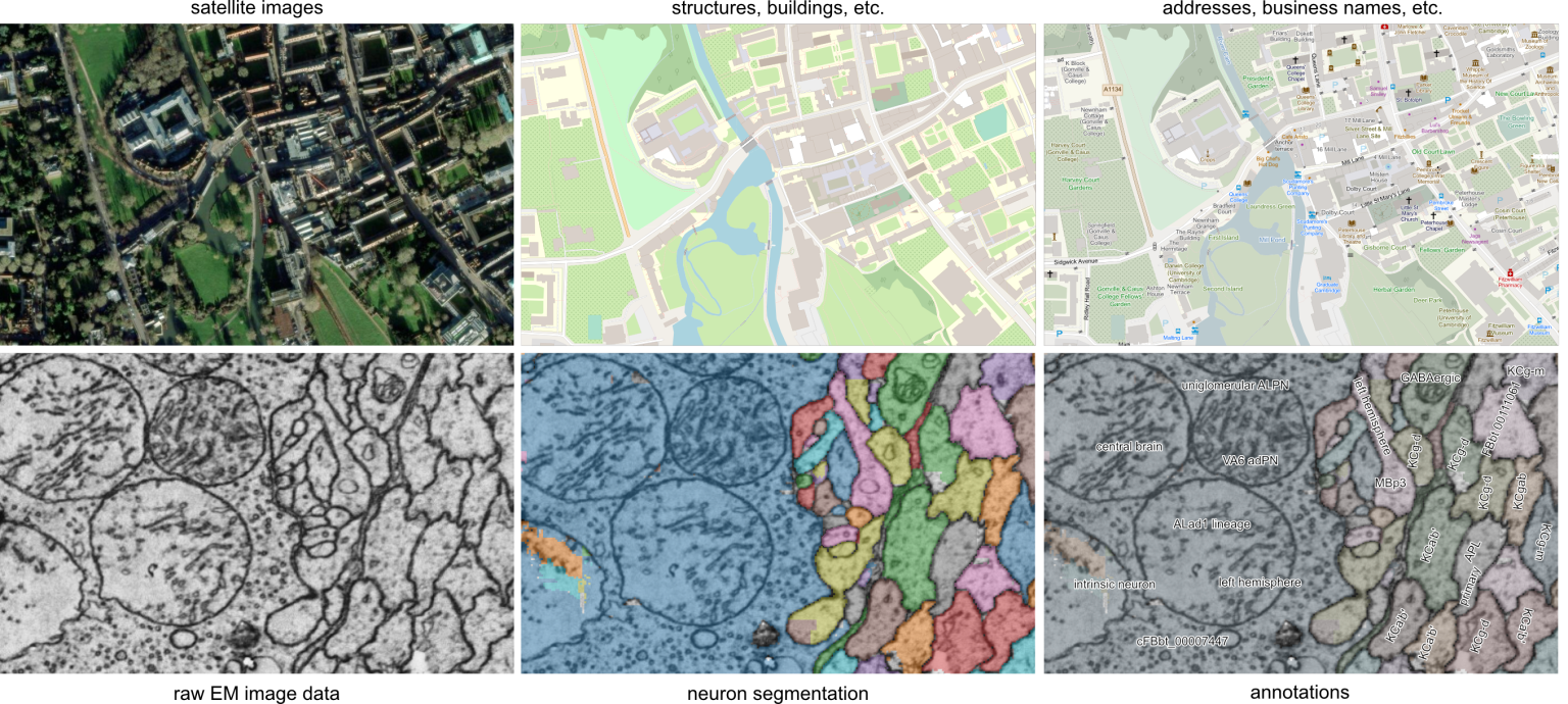
Brenner’s work was decades ahead of its time. The worm connectome had to be reconstructed by hand because digital image processing tools at that time were inadequate. Brenner and his colleagues at Cambridge’s Laboratory for Molecular Biology imaged and reconstructed all 300 neurons of the highly stereotyped worm neurons, combining eight different individuals, tracing and connecting each neuron’s spindly branches by hand. An intuitive way of illustrating this process is to compare it to satellite images of the earth (see figure below): Not only do you need to take images at extremely high resolution, you also need to determine (encircle individual areas and colorize) and annotate objects (save meta information) in order to make the helpful map. The first worm connectome paper [has been cited thousands of times](https://pubmed.ncbi.nlm.nih.gov/22462104/), and almost every year since its publication more than three decades ago, the rate of citations has increased. Still, it took neuroscientists nearly 40 years of work to go from a 300 neuron worm connectome to a 140,000 neuron fruit fly connectome.
Neurons make new connections and abandon unused synapses. Some areas even withstand the trend of declining neuron numbers over life, and we see new neurons emerge. Neuronal activity and other variables impose changes on the connectome, which influence long-term information processing and thus represent the structural equivalent of learning over time. Modern studies have revealed multiple timescales of structural plasticity, from rapid synaptic modifications occurring within minutes to slower axonal and dendritic remodeling processes that can take days or weeks. Understanding the rules governing these structural modifications may be as crucial as mapping the connections themselves, as these rules determine how the network can reconfigure itself in response to experience and environmental demands. To lean into our satellite image of the world metaphor again, we want to have a dynamic video of the world, rather than a single static picture. Despite progress in methods to study neuroplasticity ([Velicky et al., 2023](https://www.nature.com/articles/s41592-023-01936-6)), reliably tracking morphological dynamics and, through that, understanding neuroplasticity largely remains beyond what the field is capable of.
Figure 19 - Comparison of a map of the globe and connectomics A) Current Google Maps maximum zoom is approximately 1 pixel ≈ 15cm on Earth ([Google, 2014](https://cdn.tnris.org/documents/google-imagery-fact-sheet.pdf)). Intelligence experts estimate that the most advanced US military satellites can achieve resolutions of up to 6 cm per pixel. ([Richardson, 2024](https://euro-sd.com/2024/07/articles/39425/the-black-world-of-us-spy-satellites/)). An illustration in the image below ([source](https://www.firstbasesolutions.com/?faq_wd=what-does-the-photo-resolution-in-cm-mean)). Scanning the human brain at the resolution necessary to reconstruct a connectome (~20nm sized voxels necessary to trace synapses) is the same as having a map of the world 10x sharper than the current best satellites (with [6371 km radius](https://nssdc.gsfc.nasa.gov/planetary/factsheet/earthfact.html), earth’s total surface area is ~510 million km², which at 1 mm² resolution / pixel = 5.1×10²⁰ pixels. 1200 cm³ average human brain volume at 20nm isotropic voxels size is 1.5×10²⁰ voxels.). B) Figure illustrating various stages of image processing in comparison to raw satellite data: following registration (left), following segmentation and tracing (center), and following annotation (right). Source: [Schlegel, 2024](https://flyconnecto.me/2024/10/02/flywire-is-live-%f0%9f%9a%80/)

### Machine-readable figure record: `main-fig-19`
```yaml
id: main-fig-19
document_id: sobe-2025-main-ai
document_path: report.md
anchor: main-fig-19
canonical_url: https://brainemulation.mxschons.com/ai/report.md#main-fig-19
figure: "Globe/connectomics scale comparison"
assets:
- "../assets/report/main-fig-19a.png"
- "../images/connectomics-image-processing-stages.png"
data_status: unavailable_in_repository
publication_export_members:
- "images/image4.png"
- "images/image31.png"
canonical_pdf_pages:
- 127
note: "Conceptual scale comparison; prose contains the assumptions but no local computation was identified."
```
No local numeric plot input was found. The figure is a conceptual diagram, video still, or reproduction from an external publication; its caption and source remain the machine-readable provenance.
## Methods of reconstructing the brain
Reconstructing brain structure at resolutions necessary to derive the connectome pushes the boundaries of imaging techniques. On a high level, various imaging approaches use electron beams and various forms of electromagnetic waves, ranging from hard X-rays to visible light, and use one or multiple tissue processing techniques such as staining, tissue expansion, or molecular annotations. All static brain structure imaging methods perfuse the brain with chemicals to stabilize its structure during euthanization, after which it is carefully extracted and undergoes subsequent tissue preparation steps. The purpose of such tissue processing varies from increasing visibility of important structures to compensating for the resolution limitations of imaging techniques like X-ray or standard light microscopy.
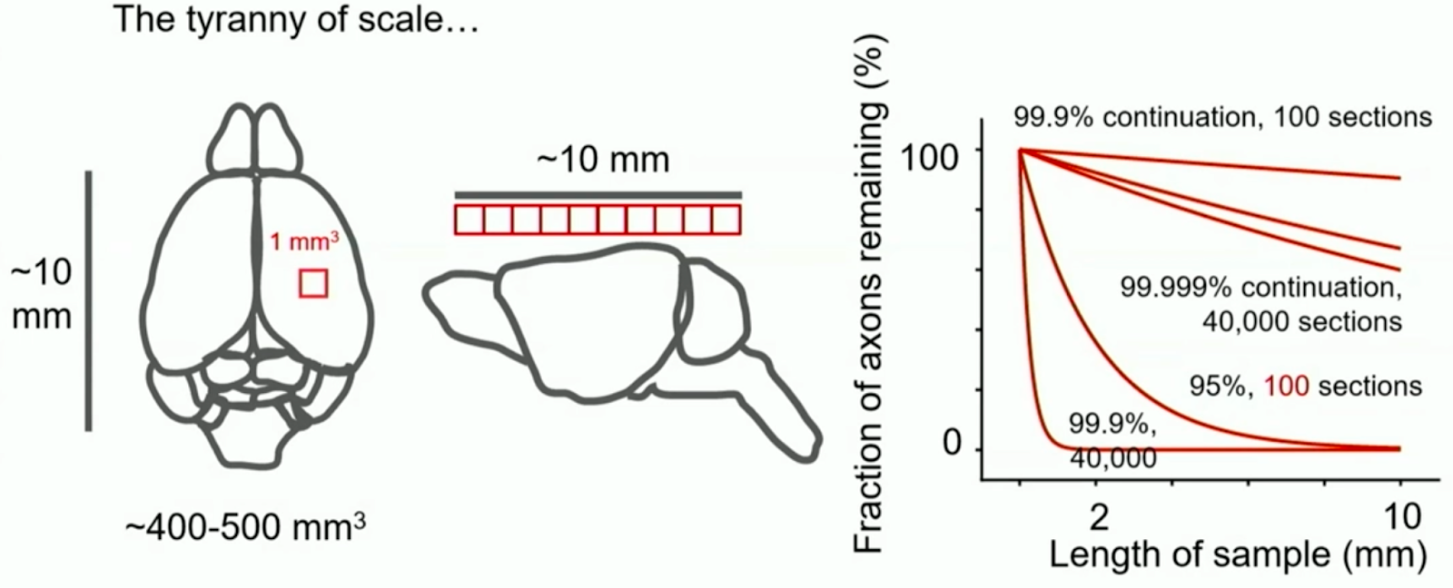
The figure below demonstrates how quickly even rare errors tracing neurons across the vast number of images can interfere with the successful reconstruction of a neuron (a 1mm long axon imaged with the above-mentioned axial resolution of 20 nm comprises 50,000 images). Tissue loss and damage increase the difficulty of following neurons across different sections during final reconstruction. Even the brains of relatively small organisms must be sliced to arrive at processable sizes that match equipment capacity, diffusion speeds, and parallelization across multiple machines. So far, 1 mm-thick samples have routinely demonstrated robust results. However, cutting brain tissue into ~1 mm slices with "ultra-smooth" vibratomy becomes increasingly difficult with bigger brains.
As we will see in the following chapter, tracing neurons via morphology relies on the high resolution and subsequent time-consuming reconstruction and error correction. If it were possible to uniquely identify the same neuron at its soma and far end, that would loosen the hampering constraint of requiring virtually error-free tracing. This is the idea of barcoding: place a uniquely identifiable molecule in each neuron that can unambiguously determine the identity of each cell. Then, even if it were impossible to trace a neuron continuously through tissue, the expressed barcode would allow correct identification of distal synapses. Loss of an entire section or slicing errors would be much less catastrophic than in any morphologic approach, as barcoding would not rely on perfect traceability.
Barcodes can come in many forms, and scientists are becoming increasingly creative, generating more ambitious variants.
Figure 20 - Replication of the Tyranny of Scale Figure from the NIH Brain Connects Workshop Series. Even at relatively low error rates, tracing accuracy deteriorates given high numbers of imaging sections with large brain volumes.
### Machine-readable figure record: `main-fig-20`
```yaml
id: main-fig-20
document_id: sobe-2025-main-ai
document_path: report.md
anchor: main-fig-20
canonical_url: https://brainemulation.mxschons.com/ai/report.md#main-fig-20
figure: "Tyranny of scale"
assets:
- "../images/tyranny-of-scale-tracing-accuracy-graph.png"
data_status: unavailable_in_repository
publication_export_members:
- "images/image47.png"
canonical_pdf_pages:
- 129
note: "Static reproduction; no local plot input was identified."
```
No local numeric plot input was found. The figure is a conceptual diagram, video still, or reproduction from an external publication; its caption and source remain the machine-readable provenance.
### Structural imaging approaches
Morphology staining approaches are the most common method in connectomics. Tissue sections are completely stained to highlight morphological features, particularly cell boundaries (membranes) and protein densities. The advantage is that “everything” is visualized, and the technique is general to any tissue type. The disadvantage is that imaging at a high enough resolution to resolve desired features is time-consuming and data-intensive. Electron microscopy, connectomics and X-ray approaches typically use osmium or other heavy metal stains, whereas antibody- or lipid-based morphology staining is used in light microscopy.
#### Electron microscopy
Electron microscopes use electron beams that are accelerated through a high voltage and are precisely guided by electromagnetic lenses to focus on a sample with nanometer precision. As these electrons interact with the sample’s atoms, various signals are generated – such as secondary electrons, backscattered electrons, or transmitted electrons – depending on the type of microscope. Specialized sensors detect these signals, which are then processed and transformed into highly detailed images revealing the sample’s structure, composition, and even atomic arrangements. For Volume Electron Microscopy (vEM), series of such 2D images are first acquired and then computationally reconstructed into 3D volumes. The imaging techniques for acquiring these series primarily fall into two categories: Transmission Electron Microscopy (TEM)-based and Scanning Electron Microscopy (SEM)-based approaches.
TEM-based vEM techniques, such as serial section TEM (ssTEM), involve physically cutting the biological sample into a series of ultra-thin sections (typically 30-100 nm thick). Each section is collected on a support grid and imaged individually in a TEM, where the electron beam passes through it to form a 2D projection image. These serial 2D images are subsequently aligned and stacked to reconstruct the 3D volume. TEM generally offers excellent lateral resolution due to the thinness of the sections and the physics of electron transmission, but its axial resolution is inherently limited by the physical thickness of each section. Advances like GridTape TEM ([Phelps et al., 2021](https://www.sciencedirect.com/science/article/pii/S0092867420316834)) further automate section handling and imaging for ssTEM, significantly increasing throughput
([Peddie et al., 2022](https://www.nature.com/articles/s43586-022-00131-9)).
SEM-based vEM techniques typically involve iteratively imaging the surface (or "block-face") of a sample within the SEM, then removing a thin layer to expose a new surface for the next image. Several approaches exist. Focused Ion Beam SEM (FIB-SEM) uses a focused ion beam (e.g., gallium) to ablate or "mill" away very thin layers (typically 5-20 nm) from the sample surface. After each layer's removal, the newly exposed block-face is imaged by the SEM using backscattered or secondary electrons. This process allows for very high axial resolution, making isotropic voxels achievable. For large-volume acquisitions, where milling proceeds over significant depths (e.g., hundreds of micrometers), the milling front can become uneven; periodic replanarization steps are often necessary to re-flatten the sample surface and maintain a consistent cutting plane. Serial Block-Face SEM (SBF-SEM) employs an ultramicrotome (a diamond knife) integrated directly inside the SEM chamber. The knife cuts a thin section (typically 25-100 nm) from the block-face, which is discarded, and the newly exposed surface is then imaged. SBF-SEM is generally faster for very large fields of view compared to FIB-SEM but offers lower axial resolution. Array Tomography (AT) involves first cutting an entire series of ultra-thin sections, collecting them in an ordered array (e.g., on a silicon wafer or specialized tape), and then imaging them sequentially in an SEM. While its z-resolution is limited by section thickness (e.g., 30-50 nm), AT uniquely allows for post-section staining, re-imaging of regions of interest, and is well-suited for correlative light and electron microscopy. For very large tissue samples, they may first be subdivided into more manageable "slabs" or ribbons, for instance using a hot knife, before serial sectioning for AT ([Peddie et al., 2022](https://www.nature.com/articles/s43586-022-00131-9)).
To accelerate the inherently slow process of SEM imaging, multi-beam SEM (mSEM) systems have been developed. As early as 2015, Zeiss produced 61-beam SEMs capable of approaching GHz data acquisition speeds ([Zeidler et al, 2015](https://onlinelibrary.wiley.com/doi/10.1111/jmi.12224)). Current state-of-the-art devices feature 91 beams ([Riedesel et al., 2019](https://eipbn.org/abstracts/2019/papers/10B-6.pdf)). In mSEM, the primary electron beam is split into multiple sub-beams, each scanning a small region of the sample in parallel to simultaneously generate images of the underlying tissue. These individually captured high-resolution images are then computationally stitched together to form a larger composite image. While mSEMs can achieve burst imaging speeds of up to 3.6 GHz (e.g., ~40 MHz per beam for a 91-beam system), the effective rate, when projected over 24/7 scanning operations considering factors like downtime and sample exchange, typically falls to 100-200 MHz. In this context, 1 Hz is equivalent to imaging one voxel per second. To put this in perspective: scanning a 500 mm³ volume of mouse brain (approximately 500 petavoxels at 10nm isotropic resolution) would take about twenty 91-beam EM systems roughly four years, assuming continuous 24/7 scanning at an effective imaging rate of 200 MHz per system.
Only a handful of facilities globally possess the multiple, high-throughput vEM systems required for such large-scale endeavors. Setup costs for a single advanced vEM instrument range between \$0.5 million and \$10 million, with similar maintenance costs over 3-5 years. Depending on uptime and specific operational context, costs per hour can range between \$1,000 and \$5,000.
Figure 21 - [Replication](https://docs.google.com/document/d/19DpNUlwU30d4IpH5A1glFVeL0uTDL7BpASdEDZ6yvWo/edit?tab=t.0#heading=h.yme2o6mykhse) of Wellcome Trust Figure on EM Datasets, data see [here](https://doi.org/10.5281/zenodo.7599974): The imaging speeds and volumes for electron microscopy in connectomics have increased substantially over time.

### Machine-readable figure record: `main-fig-21`
```yaml
id: main-fig-21
document_id: sobe-2025-main-ai
document_path: report.md
anchor: main-fig-21
canonical_url: https://brainemulation.mxschons.com/ai/report.md#main-fig-21
figure: "EM dataset scaling"
assets:
- "../assets/report/main-fig-21.png"
data_status: final_circulation_export_raster_with_contextual_current_sources
data_sources:
- "../data/current-repository/external/bosch-et-al/neuroimaging-speed.tsv"
generator: ../code/run_all_figures.py
generator_function: generate_imaging_speed
publication_export_members:
- "images/image14.png"
canonical_pdf_pages:
- 131
note: "The publication raster is retained because the current generated asset differs."
```
#### Inline contextual data (not an exact publication input): Bosch et al. dataset
```tsv
mapName released_year doi img_tech n_machines_involved species organ fov_mm3 vx_avg_nm dsSize_TB imagingRate imagingRate_perMachine
mouseRetina 2011 https://doi.org/10.1038/nature09818 SBF - SEM 1 mouse eye 0.0063 18.43169357 1.006108516 0.5263157895 0.5263157895
mouseRetina 2014 doi:/10.1038/nature13240 SBF - SEM 1 mouse eye 0.0063 18.43169357 1.006108516 0.5263157895 0.5263157895
rabbitRetina 2011 https://doi.org/10.1038/nn.2868 SBF - SEM 1 rabbit eye 0.0001053 24.39620115 0.007252066116 0.125 0.125
mouseRetina 2011 https://doi.org/10.1038/nn.2868 SBF - SEM 1 mouse eye 0.0012636 18.95116731 0.1856528926 0.1666666667 0.1666666667
mouseRetina 2011 https://doi.org/10.1038/nn.2868 SBF - SEM 1 mouse eye 0.00119625 15.32618865 0.3322916667 0.2 0.2
mouseCortex 2011 https://doi.org/10.1038/nature09802 ss - TEMCA 1 mouse brain 0.00819 9.283177667 10.2375 5 5
stainingTest 2015 https://doi.org/10.1038/ncomms8923 SBF - SEM 1 mouse brain 0.000135915 16.2865057 0.03146180556 0.3125 0.3125
mouseRetina 2016 https://doi.org/10.1038/nature18609 SBF - SEM 1 mouse eye 0.00273 16.5465353 0.6026170799 0.4 0.4
zebrafishOB_adult 2016 https://doi.org/10.1038/nn.4290 SBF - SEM 1 zebrafish brain 0.004882752 12.65148998 2.411235556 2 2
zebrafishOB_larva 2016 https://doi.org/10.1038/nn.4290 SBF - SEM 1 zebrafish brain 0.000923082776 12.88470535 0.4315361407 2 2
mouseCortex 2016 https://doi.org/10.1038/nature17192 ss - TEMCA 1 mouse brain 0.030375 8.61773876 47.4609375 8 8
flyBrain_larva 2015 https://doi.org/10.1038/nature14297 ss - TEM 1 fly brain 0.0037510605 8.971100718 5.195374654 undisclosed undisclosed
flyBrain_larva 2015 https://doi.org/10.1038/nature14297 ss - TEM 1 fly gut 0.0001781836916 8.61773876 0.2784120181 undisclosed undisclosed
flyBrain_adult 2018 https://doi.org/10.1016/j.cell.2018.06.019 ss - TEMCA 2 fly brain 0.01999077034 8.61773876 31.23557866 50 50
mouseL4 2015 https://doi.org/10.1016/j.neuron.2015.09.003 SBF - SEM 1 mouse brain 0.00051894 15.23690938 0.1466987772 undisclosed undisclosed
mouseCortex 2015 https://doi.org/10.1016/j.cell.2015.06.054 ATUM - SEM 1 mouse brain 0.000677766 8.61773876 1.059009375 1 1
zebrafishBrain_larva 2017 https://doi.org/10.1038/nature22356 ATUM - SEM 2 zebrafish brain 0.2922296108 57.57533666 1.531139503 1 1
zebrafishBrain_larva 2017 https://doi.org/10.1038/nature22356 ATUM - SEM 2 zebrafish brain 0.0545751 27.67933485 2.573520258 1 1
flyBrain_mb 2017 https://doi.org/10.7554/eLife.26975 FIB - SEM 1 fly brain 0.00024 8 0.46875 0.1550099206 0.1550099206
flyBrain_antennaLobe 2017 DOI: 10.7554/eLife.24838 ATUM - SEM 1 fly brain 0.028755 9.283177667 35.94375 8 8
flyBrain_medulla 2013 https://doi.org/10.1038/nature12450 ss - TEM 1 fly eye 0.0001790908416 9.479512636 0.21024 0.03743589744 0.03743589744
flyBrain_medulla 2015 www.pnas.org/cgi/doi/10.1073/pnas.1509820112 FIB - SEM 1 fly eye 0.000128 10 0.128 undisclosed undisclosed
nematode 2013 https://doi.org/10.1016/j.cell.2012.12.013 ss - TEM 1 nematode pharynx 0.001057119704 9.127806105 1.390032485 undisclosed undisclosed
mouseBarrelCx_P5 2020 https://www.science.org/doi/10.1126/science.abb4534 SBF - SEM 1 mouse brain 0.000545014886 15.59138249 0.1437985435 undisclosed undisclosed
mouseBarrelCx_P7 2020 https://www.science.org/doi/10.1126/science.abb4534 SBF - SEM 1 mouse brain 0.001496389778 15.59138249 0.3948124649 undisclosed undisclosed
mouseBarrelCx_P9 2020 https://www.science.org/doi/10.1126/science.abb4534 SBF - SEM 1 mouse brain 0.000865911592 15.59138249 0.2284649996 undisclosed undisclosed
mouseBarrelCx_P14 2020 https://www.science.org/doi/10.1126/science.abb4534 SBF - SEM 1 mouse brain 0.000849386874 15.59138249 0.2241050629 undisclosed undisclosed
humanCortex 2022 https://doi.org/10.1126/science.abo0924 SBF - SEM 1 human brain 0.00407589828 15.59138249 1.075398583 1.428571429 1.428571429
humanCortex 2022 https://doi.org/10.1126/science.abo0924 SBF - SEM 1 human brain 0.002887455792 15.59138249 0.761835957 1.428571429 1.428571429
macaqueCortex 2022 https://doi.org/10.1126/science.abo0924 SBF - SEM 1 macaque brain 0.003718273104 15.59138249 0.9810415648 2.5 2.5
macaqueCortex 2022 https://doi.org/10.1126/science.abo0924 SBF - SEM 1 macaque brain 0.00441049536 15.59138249 1.163679791 2.5 2.5
mouseCortex 2022 https://doi.org/10.1126/science.abo0924 SBF - SEM 1 mouse brain 0.001067553375 15.23690938 0.3017858994 undisclosed undisclosed
mouseCortex 2022 https://doi.org/10.1126/science.abo0924 SBF - SEM 1 mouse brain 0.003042213424 15.59138249 0.8026677263 undisclosed undisclosed
mouseCortex 2022 https://doi.org/10.1126/science.abo0924 SBF - SEM 1 mouse brain 0.002044994 16.2865057 0.4733782407 undisclosed undisclosed
mouseCortex 2022 https://doi.org/10.1126/science.abo0924 SBF - SEM 1 mouse brain 0.00162345984 16.2865057 0.3758008889 undisclosed undisclosed
mouseCortex 2022 https://doi.org/10.1126/science.abo0924 SBF - SEM 1 mouse brain 0.00231068944 15.59138249 0.6096600009 1.428571429 1.428571429
mouseCortex 2022 https://doi.org/10.1126/science.abo0924 SBF - SEM 1 mouse brain 0.07184308429 15.59138249 18.95531874 undisclosed undisclosed
humanCortex 2022 https://doi.org/10.1126/science.abo0924 ATUM - mSEM 1 human brain 0.101031 8.389101512 171.1229675 20 20
humanCortex 2022 https://doi.org/10.1126/science.abo0924 ATUM - mSEM 1 human brain 0.06534 8.632077786 101.5858209 20 20
flyBrain_hemibrain 2020 https://doi.org/10.7554/eLife.57443 FIB - SEM 2 fly brain 0.015625 8 30.51757813 0.5434782609 0.2717391304
mouseOBcolumn 2022 https://doi.org/10.1038/s41467-022-30199-6 SBF - SEM 1 mouse brain 0.2868446586 50 2.294757269 2 2
mouseCortex 2022 https://doi.org/10.1016/j.cell.2022.01.023 ss - TEMCA 1 mouse brain 0.00315 8.003415209 6.144471146 500 500
mouseCortex 2021 https://doi.org/10.1101/2021.07.28.454025 GridTape - autoTEM 5 mouse brain 1.048944 8.61773876 1638.975 103.9431126 20.78862253
humanCortex 2021 https://doi.org/10.1101/2021.05.29.446289 ATUM - mSEM 1 human brain 0.7 8.082480041 1325.757576 190.0057002 190.0057002
flyNerveCord 2021 https://doi.org/10.1016/j.cell.2020.12.013 GridTape - TEMCA 1 fly brain 0.0608 9.405527155 73.0725317 42.73504274 42.73504274
nematode 1986 http://www.jstor.org/stable/2990196?origin=JSTOR-pdf ss - TEM 2 nematode organism 0.052 9.283177667 65 undisclosed undisclosed
cells_FIBSEM 2020 DOI: 10.1126/science.aaz5357 FIB - SEM 1 cells 0.0001 4 1.5625 0.2 0.2
cells_FIBSEM 2021 https://doi.org/10.1016/j.cell.2021.03.035 FIB - SEM 1 cells 7.79e-06 8 0.01521484375 undisclosed undisclosed
cells_FIBSEM 2021 https://doi.org/10.1016/j.cell.2021.03.035 FIB - SEM 1 cells 2.32724448e-05 8 0.04545399375 undisclosed undisclosed
cells_FIBSEM 2021 https://doi.org/10.1016/j.cell.2021.03.035 FIB - SEM 1 cells 1.60992e-05 8 0.03144375 undisclosed undisclosed
cells_FIBSEM 2021 https://doi.org/10.1016/j.cell.2021.03.035 FIB - SEM 1 cells 4.88736e-05 8 0.09545625 undisclosed undisclosed
cells_FIBSEM 2021 https://doi.org/10.1016/j.cell.2021.03.035 FIB - SEM 1 cells 3.9544e-05 8 0.077234375 undisclosed undisclosed
cells_FIBSEM 2021 https://doi.org/10.1016/j.cell.2021.03.035 FIB - SEM 1 cells 3.6e-05 8 0.0703125 undisclosed undisclosed
cells_FIBSEM 2021 https://doi.org/10.1016/j.cell.2021.03.035 FIB - SEM 1 cells 9.504e-06 4.376736725 0.1133587786 undisclosed undisclosed
cells_FIBSEM 2021 https://doi.org/10.1016/j.cell.2021.03.035 FIB - SEM 1 cells 7.8e-06 4.376736725 0.09303435115 undisclosed undisclosed
mouse_cochlea 2021 https://doi.org/10.1016/j.celrep.2020.108551 SBF - SEM 1 mouse brain 0.0050828 16.91538112 1.050165289 1 1
mouse_cochlea 2021 https://doi.org/10.1016/j.celrep.2020.108551 SBF - SEM 1 mouse brain 0.0030606336 19.30978769 0.425088 0.6666666667 0.6666666667
mouse_cochlea 2021 https://doi.org/10.1016/j.celrep.2020.108551 SBF - SEM 1 mouse brain 0.003094848 19.30978769 0.42984 0.5 0.5
mouse_glomerulus 2018 DOI: 10.1038/s41467-017-02560-7 SBF - SEM 1 mouse brain 0.00648 17.55276591 1.198224852 0.3333333333 0.3333333333
mouse_glomerulus 2018 DOI: 10.1038/s41467-017-02560-7 SBF - SEM 1 mouse brain 0.001296 17.55276591 0.2396449704 0.3333333333 0.3333333333
ciona_ns 2013 https://doi.org/10.7554/eLife.16962 ss - TEM 1 ciona nervous_system 0.002025 9.616659441 2.276943835 undisclosed undisclosed
platynereis_eye 2014 https://doi.org/10.7554/eLife.02730 ss - TEM 1 platynereis brain 0.001568 8.210733515 2.832697422 undisclosed undisclosed
zebrafinch_cortex 2017 https://doi.org/10.7554/eLife.24364 SBF - SEM 1 zebrafinsh brain 0.002121812 15.19594767 0.604677116 2.127659574 2.127659574
zebrafinch_bs 2018 https://doi.org/10.1038/nmeth.4206 SBF - SEM 1 zebrafinsh spinal cord 0.0010763126 11.74460292 0.6643904938 undisclosed undisclosed
zebrafish_larva 2022 https://doi.org/10.1038/s41592-022-01621-0 SBF - SEM 1 zebrafish brain 0.057960603 16.98499252 11.82869449 2.074336155 2.074336155
zebrafish_spinalcord 2018 https://doi.org/10.1016/j.celrep.2018.05.023 SBF - SEM 1 zebrafish spinal cord 0.001133532 11.93717162 0.6663915344 5 5
```
#### Figure-generation source map (valid Python; not standalone plotting code)
```python
GENERATOR_PATH = "../code/run_all_figures.py"
SOURCE_FUNCTION = 'generate_imaging_speed'
SELECTED_SOURCE_LINES = (
"imaging_speed_df['imagingRate_perMachine'] = pd.to_numeric(",
"imaging_speed_df['imagingRate_perMachine'], errors='coerce'",
"data=imaging_speed_df, x='released_year', y='imagingRate_perMachine',",
"data=imaging_speed_df, x='released_year', y='dsSize_TB',",
)
```
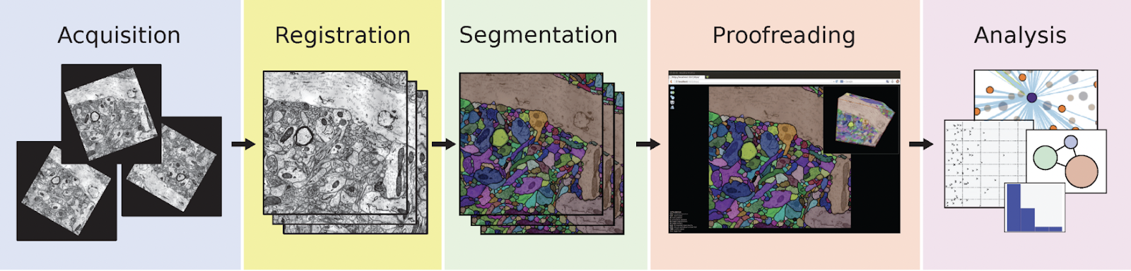
Figure 22 - Replication of Figure 15 in [Mineault et al, 2024](https://arxiv.org/abs/2411.18526), for a complete connectomics pipeline overview.
### Machine-readable figure record: `main-fig-22`
```yaml
id: main-fig-22
document_id: sobe-2025-main-ai
document_path: report.md
anchor: main-fig-22
canonical_url: https://brainemulation.mxschons.com/ai/report.md#main-fig-22
figure: "Connectomics pipeline"
assets:
- "../images/connectomics-pipeline-mineault-2024.png"
data_status: unavailable_in_repository
publication_export_members:
- "images/image23.png"
canonical_pdf_pages:
- 131
note: "Diagram reproduced after Mineault et al. (2024)."
```
No local numeric plot input was found. The figure is a conceptual diagram, video still, or reproduction from an external publication; its caption and source remain the machine-readable provenance.
#### Expansion Microscopy with Dense Labeling
In 2015, Chen et al. introduced expansion microscopy (ExM), a revolutionary technique achieving initial resolutions as fine as 70 nm. Electron microscopy (EM) is constrained by physics to a resolution limit of 0.23 nm ([Penczek, 2010](https://doi.org/10.1016/S0076-6879(10)82003-8)). In contrast, traditional light microscopy is constrained to a lateral resolution of ~250 nm and an axial resolution of ~550 nm by the diffraction limit ([Huang et al., 2010](https://www.cell.com/cell/fulltext/S0092-8674(10)01420-0)). Expansion Microscopy effectively circumvents the diffraction limit by isotropically physically expanding the tissue sample rather than attempting to improve the microscope's resolving power. Since then, multiple authors have demonstrated the dense labeling of protein ([M’Saad and Bewersdorf, 2020](https://www.nature.com/articles/s41467-020-17523-8); [M’Saad et al., 2022](https://doi.org/10.1101/2022.04.04.486901)) and lipid components ([Karagiannis et al., 2019](https://doi.org/10.1101/829903); [Shin et al, 2025](https://www.nature.com/articles/s41467-025-56641-z)).
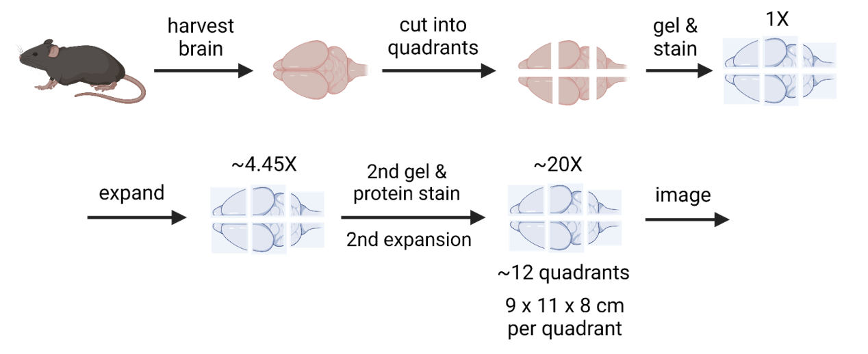
ExM pipelines physically expand biological samples by embedding them in swellable hydrogels (see figure). Routine expansion protocols can expand brains between 4- and 16-fold, while recent iterative and non-iterative expansion advances allow expansion up to 40-fold and beyond. Brain tissue sections (typically 50-70 μm thick) are first fixed, then embedded in a first hydrogel. After denaturation, the sample expands in water. The sample is then re-embedded in a second neutral gel, followed by a third expansion gel with a non-cleavable crosslinker. During this process, proteins can be labeled with antibodies and pan-stained with fluorescent dyes to reveal ultrastructure. For instance, the final expansion described by M’Saad et al. achieves approximately 24-fold total enlargement. This enables the resolution of features as small as ~15 nm in the pre-expanded sample using standard confocal microscopes, effectively bypassing the diffraction limit ([M’Saad et al., 2022](https://doi.org/10.1101/2022.04.04.486901)). The entire process takes 4-5 days from initial fixation to final imaging, with the key advantage that no specialized equipment, such as expensive electron microscopes, beyond a standard confocal microscope, is needed.
Figure 23 - Expansion Microscopy Process. Illustration of stepwise processing of brain tissue in the context of expansion microscopy. Credits to Eon Systems PBC
### Machine-readable figure record: `main-fig-23`
```yaml
id: main-fig-23
document_id: sobe-2025-main-ai
document_path: report.md
anchor: main-fig-23
canonical_url: https://brainemulation.mxschons.com/ai/report.md#main-fig-23
figure: "Expansion microscopy process"
assets:
- "../images/expansion-microscopy-process-diagram.png"
data_status: unavailable_in_repository
publication_export_members:
- "images/image29.png"
canonical_pdf_pages:
- 132
note: "Conceptual process diagram."
```
No local numeric plot input was found. The figure is a conceptual diagram, video still, or reproduction from an external publication; its caption and source remain the machine-readable provenance.
Figure 24 - Replication of Figure by [M’Saad et al., 2022](https://www.biorxiv.org/content/10.1101/2022.04.04.486901v2.full.pdf): pan-ExM-t workflow for mouse brain tissue sections. (a-f) Experimental workflow. (g): Timeline summarizing the protocol. Abbreviations: FA: formaldehyde; AAm: acrylamide; NaOH: sodiumhydroxide; DHEBA: N,N′-(1,2-dihydroxyethylene) bis-acrylamide; SDS: sodium dodecyl sulfate; PBS-T:0.1% (v/v) TX-100 in PBS; ROI: region of interest.

### Machine-readable figure record: `main-fig-24`
```yaml
id: main-fig-24
document_id: sobe-2025-main-ai
document_path: report.md
anchor: main-fig-24
canonical_url: https://brainemulation.mxschons.com/ai/report.md#main-fig-24
figure: "pan-ExM-t workflow"
assets:
- "../assets/report/main-fig-24.png"
data_status: unavailable_in_repository
publication_export_members:
- "images/image42.png"
canonical_pdf_pages:
- 133
note: "External reproduction after M’Saad et al. (2022)."
```
No local numeric plot input was found. The figure is a conceptual diagram, video still, or reproduction from an external publication; its caption and source remain the machine-readable provenance.
Expansion microscopy is beginning to bridge the gap between the molecular specificity of light microscopy and the synaptic resolution required for dense connectomics. Two complementary dense-labeling strategies have been demonstrated in brain tissue for ExM-based ultrastructural contrast: (i) pan-protein labeling (pan-ExM/pan-ExM-t) that produces dense, EM-like protein-density contrast and is compatible with immunostaining ([M’Saad et al., 2022](https://www.biorxiv.org/content/10.1101/2022.04.04.486901v1)), and (ii) dense, continuous membrane labeling (umExM) for nanoscale visualization of membranes in intact tissues ([Shin et al., 2024](https://www.biorxiv.org/content/10.1101/2024.03.07.583776v1)).
A recent proof-of-principle for dense light-microscopy connectomics is LICONN ([Tavakoli et al., 2025](https://www.nature.com/articles/s41586-025-08985-1)). The method uses pan‑protein labeling with iterative expansion, combined with a standard spinning‑disk confocal microscope for imaging and readout. In mouse cortex and hippocampus samples, LICONN demonstrated an effective optical resolution of ~20 nm laterally and ~50 nm axially (~9.7 × 9.7 × 25.9 nm³ voxel size), and an effective imaging throughput of ~17 MHz (~0.001 mm³ imaged over 6.5 hours). For reconstruction, Tavakoli et al. adopted a pipeline directly from EM connectomics, using automated segmentation with flood‑filling networks (FFNs) followed by manual proofreading, yielding reconstruction accuracy comparable to state‑of‑the‑art EM pipelines ([Tavakoli et al., 2025](https://www.nature.com/articles/s41586-025-08985-1)).
Figure 25 - Replication of Figure 1 in [Collins et al., 2024](https://arxiv.org/abs/2405.10488). Comparison of raw image data in serial section transmission electron microscopy (top) and expansion confocal light microscopy (bottom). Note the 1-2 order of magnitude higher resolution. Image from Collins et al.

### Machine-readable figure record: `main-fig-25`
```yaml
id: main-fig-25
document_id: sobe-2025-main-ai
document_path: report.md
anchor: main-fig-25
canonical_url: https://brainemulation.mxschons.com/ai/report.md#main-fig-25
figure: "EM versus expansion microscopy"
assets:
- "../assets/report/main-fig-25.png"
data_status: unavailable_in_repository
publication_export_members:
- "images/image32.png"
canonical_pdf_pages:
- 134
note: "External reproduction after Collins et al. (2024)."
```
No local numeric plot input was found. The figure is a conceptual diagram, video still, or reproduction from an external publication; its caption and source remain the machine-readable provenance.
Unlike EM pipelines, LICONN natively supports molecular annotation in the same high‑resolution volume. Presynaptic and excitatory postsynaptic markers (e.g., bassoon and SHANK2) and inhibitory postsynaptic markers (gephyrin) are imaged together with the dense structural channel, enabling direct classification of synapses. Importantly, astrocytic connexin‑43 labeling reveals gap junctions, allowing electrical coupling to be mapped at scale -- something that is typically difficult to recover with EM alone. Furthermore, because the structural and molecular channels are perfectly aligned, the data can be used to train deep learning models that predict molecular locations from the structural channel alone. The authors demonstrated this by training predictors for presynaptic and postsynaptic markers, achieving high accuracy on held-out data. This strategy can significantly reduce the number of staining rounds required when scaling up imaging to larger volumes, as the structural map can be used to infer select features.
Throughput is the main limitation at present. LICONN’s ~17‑MHz rate is well below multi‑beam EM, but those EM throughputs depend on scarce, multi‑million‑dollar systems; by contrast, the LICONN result came from a standard, relatively inexpensive spinning‑disk setup. The current throughput is thus a function of the chosen readout, not a fundamental limit of the sample preparation, which is not tied to any specific imaging modality. The clear path to scaling, therefore, involves pairing LICONN-like sample preparation with optics designed for high-speed volumetric imaging. Such a combination could achieve EM-competitive throughputs while preserving the molecular annotation that EM lacks. This potential to match EM speed and resolution on accessible equipment makes dense ExM a compelling route to scalable molecularly annotated connectomics.
#### X-ray synchrotron approaches
X-ray synchrotron approaches use high-energy X-rays to visualize tissue architecture and cellular features. The method can leverage the natural contrast between different cellular components based on their electron density and elemental composition for minimal preparation requirements. It can also use heavy metal stains like osmium or gold to enhance the contrast of specific features, particularly membranes and synaptic proteins. These stains also increase acquisition time ([Ahn et al., 2013](https://www.mdpi.com/1420-3049/18/5/5858); [Depannemaecker et al., 2019](https://pubs.acs.org/doi/10.1021/acschemneuro.9b00290)). Special chemicals can be leveraged to increase radiation resistance of samples ([Bosch et al., 2023](https://doi.org/10.1101/2023.11.16.567403)). Imaging is also generally non-destructive, meaning the same sample can be imaged through other modalities.
Spatial resolutions – not limited by diffraction, but rather by the x-ray cross section of elements with low atomic numbers in unstained samples and, more generally, by the risk of damage caused by high x-ray radiation doses – down to roughly 10 nm are theoretically possible in frozen hydrated samples ([Howells et al., 2009](https://www.sciencedirect.com/science/article/abs/pii/S0368204808001424?via%3Dihub)). The primary advantages are that the high penetration depth of X-rays allows for imaging of large tissue volumes (several mm³) at resolutions approaching 30 nm ([Stevens et al., 2020](https://www.osti.gov/biblio/1821173); [Du et al., 2021](https://journals.iucr.org/j/issues/2021/02/00/jo5064/)).
The drawbacks are also multiple, however. X-ray approaches for structural brain mapping are far less developed than their EM and light-microscopy counterparts. This is partly because imaging generally requires access to a beamline at a synchrotron facility, with beamlines heavily oversubscribed. Scalability-wise, although simulations are encouraging, significant progress is needed, particularly in improved detectors, before scalability could be sufficient for imaging whole mammalian brains ([Collins, 2023](https://logancollinsblog.com/wp-content/uploads/2023/02/feasibility-of-mapping-the-human-brain-with-expansion-x-ray-microscopy-logan-thrasher-collins-6.pdf); [Du et al., 2021](https://journals.iucr.org/j/issues/2021/02/00/jo5064/index.html)). Recent developments include sub-100 nm imaging and dense reconstruction of fly and mouse brain tissue using x-ray holographic nano-tomography ([Kuan et al., 2020](https://www.nature.com/articles/s41593-020-0704-9)), correlative studies involving in-vivo recordings, x-ray synchrotron microtomography and electron microscopy ([Bosch et al., 2022](https://www.nature.com/articles/s41467-022-30199-6)), the establishment of the SYNAPSE consortium for imaging a whole human brain at 300 nm resolution ([Stampfl et al., 2023](https://www.sciencedirect.com/science/article/pii/S0370157322003933)), the development of protocols for highly multiplexed x-ray fluorescence ([Strotton et al., 2023](https://www.nature.com/articles/s41592-023-01977-x)) and successful imaging of individual synapses through x-ray ptychography ([Bosch et al., 2023](https://doi.org/10.1101/2023.11.16.567403)).
For a visualization of X-ray synchrotron approaches, see Figure 1 in [Dyer et al., 2017](https://www.eneuro.org/content/4/5/ENEURO.0195-17.2017). Due to copyright constraints, we cannot replicate this image here.
### Barcoding approaches
Protein barcoding for connectomics emerged from the convergence of two key technological advances: site-specific DNA recombination and fluorescent protein engineering. The watershed moment came with Brainbow in 2007, which leveraged Cre/lox recombination to stochastically express different ratios of fluorescent proteins in individual neurons. This approach achieved roughly 100 distinguishable color combinations through the differential expression of red, green, and blue fluorescent proteins. The initial proof-of-concept in mice demonstrated the potential for unique cellular labeling, though it also revealed fundamental challenges in achieving consistent expression levels and maintaining color fidelity across large tissue volumes. Expression in different cell types is uneven, trafficking of these proteins is uneven, and fluorescent staining is uneven. A distal axon may display a slightly different barcode than the soma within the same neuron, complicating correct identification. Subsequent iterations expanded the technique to other model organisms, notably Drosophila, while attempting to address these limitations through improved fluorescent proteins and more sophisticated genetic designs ([Livet et al., 2007](https://www.nature.com/articles/nature06293), [Pan et al., 2011](https://doi.org/10.1101/pdb.prot5546), [Cai et al., 2013](https://doi.org/10.1101/pdb.prot5546), [Leiwe et al., 2024](https://www.nature.com/articles/s41467-024-49455-y))
The most advanced approaches combine three key elements: genetic targeting, protein-based labeling, and multi-round imaging. In current protocols, viral vectors deliver genetic constructs encoding multiple protein markers, each under the control of an independent promoter. These markers can be fluorescent proteins, epitope tags, or engineered protein scaffolds designed for subsequent antibody labeling (see figure by [Serrano, 2022](https://www.nature.com/articles/s41568-022-00500-2?fromPaywallRec=true)). The overall process requires multiple rounds of staining, washing, and imaging.
Such barcoding approaches face three distribution problems when delivery is carried out via viral vectors:
1. Distribution to all neurons.
2. Even distribution among all neurons.
3. Distribution within neurons.
For a visualization of barcoding, see Figure 1 in [Serrano, 2022](https://www.nature.com/articles/s41568-022-00500-2?fromPaywallRec=true). Due to copyright constraints, we cannot print the figure here.
In 2020, Shen et al. combined Brainbow with multi-round immunolabeling in expansion microscopy, which allowed the unique identification of neurons and reconstruction of their structure, including imaging up to 15 different stained targets ([Shen et al., 2020](https://www.nature.com/articles/s41467-020-18422-8)). Notably, super-multicolor Tetbow allows reconstruction despite two sections of a neuron being separated, beginning to leverage the core strength of barcoding ([Leiwe et al. 2024](https://www.nature.com/articles/s41467-024-49455-y)). In principle, methods like Tetbow could scale to whole-brain connectomics when combined with expansion microscopy, pan-protein, and/or lipid staining.
However, achieving whole-brain connectomics using barcoding is not currently possible. The focused research organization (FRO) [E11](https://e11.bio/) is actively working on advancing barcoding technologies for whole mammalian brains.
The theoretical limits of protein barcoding intersect with fundamental biological constraints and technical capabilities. In mammalian brains, where individual neurons form between 8,000 and 30,000 synapses (though individual connections between neurons can consist of up to 60 synapses or more – even if a neuron makes 10,000 synapses with other neurons, it may connect to only a few thousand unique neurons), the mathematics of unique identification become particularly challenging. With a 25-bit binary code (2²⁵ combinations), statistical analysis reveals that in a human brain of 80 billion neurons, approximately 10 million neurons (0.02%) would share a barcode and at least one synaptic connection. While this error rate might seem problematic, it compares favorably with current electron microscopy reconstruction error rates, particularly considering that spatial information can help resolve ambiguous cases. It is important to note that whether state-of-the-art barcoding methodology can capture most neurons and especially most synapses will need to be verified in statistical comparisons against “ground-truth” electron microscope data in small, similar reconstructed samples.
Reaching almost all neurons with the viral vectors carrying the barcodes is difficult. This will require further breakthroughs in delivery, such as the intravenous bCap1 AAV capable of reaching 5-20% of cells in the brain. ([Dyno Therapeutics, n.d.](https://products.dynotx.com/bcap1/)) Various virus-based platforms (lyssavirus, Sindbis, HSV, etc.), better intravenous delivery, high-density intra-CNS injections, and creative approaches to multi-site injection throughout the brain will be required – or perhaps all four simultaneously.
Notably, nucleic acid barcoding approaches exist, where unique RNA/DNA barcodes (typically 15-30 nucleotides) are introduced into neurons using viral vectors or genetic engineering and then use sequencing as a readout. The field emerged from spatial transcriptomics methods developed in the 2010s. The transition to connectomics applications began with MAPseq ([Kebschull et al., 2016](https://doi.org/10.1016/j.neuron.2016.07.036)), which introduced high-throughput projection mapping, tracing where neurons from one brain region send their axons, without detailing individual synaptic connections. For connectivity attempts (BRICseq): Although not yet working at scale, there are current efforts to barcode neurons and transform connectomics from an imaging problem to a sequencing and analysis problem ([Huang, 2020](https://www.cell.com/cell/pdf/S0092-8674(20)30624-3.pdf)). Most recently, ExBarSeq ([Goodwin, 2022](https://www.biorxiv.org/content/10.1101/2022.07.31.502046v1)) combined barcoding with expansion microscopy to improve spatial resolution to ~20 nm. However, these methods remain more powerful for projection mapping than detailed connectivity analysis. Current throughput for projection mapping reaches 100,000+ neurons per experiment. BARseq, for instance, employs in situ sequencing of both endogenous mRNAs and synthetic RNA barcodes to infer long-range projections of neurons across whole mouse forebrain hemispheres, analyzing millions of cells ([Chen et al, 2024](https://www.nature.com/articles/s41586-024-07221-6)). In contrast, detailed connectivity mapping remains limited to hundreds of neurons due to challenges in reliably getting barcodes to and reading them from synapses.
## Data storage and processing
### Storage & Bandwidth
While high-throughput imaging of mammalian brains demands extraordinarily effective bandwidths, existing technology can largely meet these requirements, especially when combined with modern compression methods.
A human brain is roughly 1000-1400 cm³, and such a volume, if imaged at 10 nm isotropic resolution, represents roughly 1.2 zettavoxels. Assuming 2 bytes per voxel and a total acquisition time of about a year, grayscale imaging thus requires a total effective bandwidth of about 600 terabits/s. Multiplexed imaging scales bandwidth requirements linearly with the number of colors; thus, streaming 30-color imaging data requires a total bandwidth of roughly 18 petabits/s. However, state-of-the-art compression methods already demonstrate a 128x reduction in data size without compromising subsequent reconstruction ([Li et al., 2024](https://doi.org/10.1007/978-3-031-77786-8_16)). Thus, data compression at the source could see practical bandwidth requirements decrease to about 140 terabits/s for 30-color imaging and about 5 terabits/s for grayscale imaging. Beyond these initial compression approaches, as our understanding of neural tissue matures, additional representations such as connectivity graphs and neuron skeletons could complement the detailed data, potentially offering further significant reductions in storage requirements. However, for early whole-brain reconstructions, preserving sufficient raw data to resolve subcellular structures, including synaptic vesicles and cellular organelles, will likely remain essential, as it is not yet clear which biological details are essential for faithful emulation.
Bandwidth requirements thus represent an important challenge, particularly if no compression is used. However, they are not far beyond what existing technology enables in fields such as high-energy physics. Indeed, experiments within the LHC at CERN can produce roughly a petabyte (that is, eight petabits) of raw data per second, with various filtering and compression algorithms within the sensor decreasing the effective data rate to a more manageable 50 terabytes (400 terabits) per second ([Radovic et al., 2018](https://www.nature.com/articles/s41586-018-0361-2)). Such high data rates, of course, require highly performant networking infrastructure, but that too is not far beyond current capabilities: Google data centers, for example, have demonstrated within-datacenter bandwidths of up to 13 petabits/s ([Vahdat, 2024](https://cloud.google.com/blog/products/networking/speed-scale-reliability-25-years-of-data-center-networking)). As long as compression is used and processing happens mostly within a data center co-located with the imaging facility, imaging bandwidth should thus not represent a fundamental bottleneck to efforts aiming to image a whole human brain in roughly a year, provided the level of investment is sufficient.
Figure 26 - Bandwidth Requirements by Resolution and Channel Count. Effective total bandwidth requirements for human brain imaging in less than one year at 10 nm isotropic resolution. (over one year)

### Machine-readable figure record: `main-fig-26`
```yaml
id: main-fig-26
document_id: sobe-2025-main-ai
document_path: report.md
anchor: main-fig-26
canonical_url: https://brainemulation.mxschons.com/ai/report.md#main-fig-26
figure: "Multiplexed imaging bandwidth"
assets:
- "../assets/report/main-fig-26-publication.png"
data_status: final_circulation_export_raster_with_contextual_current_sources
data_sources:
- "../data/legacy/bandwidth-scaling-multiplexed-imaging.csv"
generator: ../code/run_all_figures.py
generator_function: generate_bandwidth_scaling
publication_export_members:
- "images/image43.png"
canonical_pdf_pages:
- 140
```
#### Inline contextual data (not an exact publication input): bandwidth estimates
```tsv
resolution_nm 1-color 5-color 10-color 15-color 20-color 25-color 30-color
10 5.5e14 3.2e15 5.8e15 8.5e15 1.15e16 1.45e16 2.0e16
15 2.2e14 9.0e14 1.9e15 3.2e15 4.2e15 4.8e15 5.5e15
25 3.8e13 2.0e14 3.8e14 5.2e14 7.2e14 1.05e15 1.25e15
50 5.0e12 2.5e13 5.5e13 8.5e13 1.5e14 1.6e14 1.9e14
100 5.0e11 3.0e12 6.0e12 9.0e12 1.2e13 1.5e13 1.8e13
```
#### Figure-generation source map (valid Python; not standalone plotting code)
```python
GENERATOR_PATH = "../code/run_all_figures.py"
SOURCE_FUNCTION = 'generate_bandwidth_scaling'
SELECTED_SOURCE_LINES = (
'def generate_bandwidth_scaling():',
'# Resolution in nm vs bandwidth in bits/s for different numbers of multiplexed colors',
'bandwidth_data = {',
"'resolution_nm': [10, 15, 25, 50, 100],",
"'1-color': [5.5e14, 2.2e14, 3.8e13, 5.0e12, 5.0e11],",
"'5-color': [3.2e15, 9.0e14, 2.0e14, 2.5e13, 3.0e12],",
"'10-color': [5.8e15, 1.9e15, 3.8e14, 5.5e13, 6.0e12],",
"'15-color': [8.5e15, 3.2e15, 5.2e14, 8.5e13, 9.0e12],",
"'20-color': [1.15e16, 4.2e15, 7.2e14, 1.5e14, 1.2e13],",
"'25-color': [1.45e16, 4.8e15, 1.05e15, 1.6e14, 1.5e13],",
"'30-color': [2.0e16, 5.5e15, 1.25e15, 1.9e14, 1.8e13],",
'bandwidth_df = pd.DataFrame(bandwidth_data)',
'# Use extended categorical colors',
'bw_colors = {',
"'1-color': EXTENDED_CATEGORICAL[0],",
"'5-color': EXTENDED_CATEGORICAL[1],",
"'10-color': EXTENDED_CATEGORICAL[2],",
"'15-color': EXTENDED_CATEGORICAL[3],",
"'20-color': EXTENDED_CATEGORICAL[4],",
"'25-color': EXTENDED_CATEGORICAL[5],",
"'30-color': EXTENDED_CATEGORICAL[6],",
'for col in bandwidth_df.columns[1:]:',
"ax.plot(bandwidth_df['resolution_nm'], bandwidth_df[col], 'o-', label=col,",
'color=bw_colors[col], linewidth=2, markersize=10)',
"ax.grid(True, which='major', linestyle='--', alpha=0.6, color=COLORS['grid'])",
"ax.grid(True, which='minor', linestyle='--', alpha=0.3, color=COLORS['grid'])",
"save_figure(fig, 'brain-imaging-bandwidth-requirements')",
)
```
Depending on the compression factor, the data storage necessary for a human connectome would be on the order of 1 Peta to 100 Exabytes, with an additional 2-3x factor to accommodate for backup infrastructure. Petabyte storage capacity is common for small to mid-sized data centers. Most large data centers operated by commercial providers do not disclose their official capacity, but can store up to several exabytes (10¹⁸) of data ([Blackblaze, 2024](https://baxtel.com/news/backblaze-unveils-its-us-east-data-center-a-peek-into-1-3-exabytes-of-raw-storage-capacity)). The European Centre for Medium-Range Weather Forecasts (ECMWF) generates 400 terabytes of new data daily and processes this with previous dates to make predictions ([ECMWF, 2024](https://www.ecmwf.int/en/about/media-centre/key-facts-and-figures)). Companies like ByteDance process over 500 PB/day ([Wu et al., 2024](https://dl.acm.org/doi/10.14778/3685800.3685804)) while the most prominent actors, such as Google, Meta, or Microsoft, do not disclose official numbers. For 2025, the total globally available digital storage capacity is estimated to be around 16 zettabytes ([Statista Inc., 2021](https://www.statista.com/statistics/1185900/worldwide-datasphere-storage-capacity-installed-base/)).
### Neuron Reconstruction
Neuron reconstruction aims to recreate the three-dimensional connectome from the vast quantities of microscopy data produced through imaging. This complex process generally involves three main stages: data preparation (including registration), automated segmentation and tracing, and meticulous proofreading. Each stage presents unique challenges and opportunities for automation.
The first critical step is data preparation, where raw image data is processed for downstream analysis. A key bottleneck here is registration: aligning adjacent scans to ensure spatial consistency of neural structures. Misalignments, often caused by imaging artifacts or slight sample movements, are a dominant cause of errors in subsequent automated neuron reconstructions ([Popovych et al., 2024](https://www.nature.com/articles/s41467-023-44354-0)). Poor alignment can make it impossible for algorithms to correctly follow fine neurites across section boundaries. Fortunately, recent advancements in machine learning have significantly improved alignment accuracy, with algorithms now addressing artifact removal, de-warping, and noise reduction, in some cases reducing genuine misalignments to as low as 0.06% of image pairs ([Popovych et al., 2024](https://www.nature.com/articles/s41467-023-44354-0); [Scheffer et al., 2020](https://elifesciences.org/articles/57443)).
Once the data is prepared, the process moves to segmentation of cell boundaries and tracing of neuron skeletons (axons and dendrites). This is how the initial 3D shapes of neurons and their potential connectivity are computationally derived. Historically, manual tracing and segmentation were the only options, but these are prohibitively costly for large volumes, averaging around 11.2 hours per neuron in early dense reconstructions
([Zheng et al., 2018](https://www.sciencedirect.com/science/article/pii/S0092867418307876#app2)). Modern approaches heavily rely on automated techniques. Convolutional neural networks, such as U-Nets, can learn from relatively sparse training data to perform tasks like segmentation and synapse classification. For dense segmentation, a range of architectures – including U-Nets ([Lee et al., 2017](https://arxiv.org/abs/1706.00120)), flood-filling networks ([Januszewski et al., 2018](https://www.nature.com/articles/s41592-018-0049-4)), and embedding-based ones ([Lee et al., 2022](https://doi.org/10.1109/TMI.2021.3097826)) – have become state-of-the-art, achieving high precision in identifying which voxels belong to the same neuron. While some of these methods can be computationally intensive, ongoing architectural modifications and algorithmic refinements continue to improve efficiency and performance across the board.
Despite the capabilities of current automated segmentation algorithms, errors inevitably occur. These can be "split" errors (a single neuron incorrectly broken into multiple pieces) or "merge" errors (different neurons incorrectly joined). Correcting these errors requires proofreading, which currently represents the most significant time and cost bottleneck in EM-based connectomics, especially for dense reconstruction of complex mammalian neurons from large-scale datasets like serial section TEM (ssTEM). The human labor involved in correcting such errors is substantial. For instance, proofreading the local axonal arbor of a single mouse cortical pyramidal neuron – often considered a benchmark for the most challenging structures to trace – from a petascale EM volume (e.g., the MICrONS dataset) is estimated to take approximately 40 person-hours (T. Macrina, personal communication, 2025). This translates to direct proofreading costs of around \$400 per neuron (assuming outsourced proofreader costs of \$10/hr), though the experienced cost for a user engaging a reconstruction service can be higher, in the range of \$500-\$1000 per neuron. It's important to note these estimates often benchmark against challenging neuron types like pyramidal cells (which have extensive and fine axonal arbors) and typically focus on local arbors, with costs potentially varying for simpler neurons or different reconstruction targets. The quality of the initial imaging and automated reconstruction also heavily influences proofreading effort; imaging defects, such as missing sections, are a primary cause of errors that necessitate manual correction.
The scale of this challenge is significant: given current proofreading costs, the total proofreading expenditure for an entire mouse brain could reach upwards of \$1 billion ([Jefferis et al., 2023](https://wellcome.org/reports/scaling-connectomics)). It’s also worth noting that the difficulty of proofreading also varies across species; for example, researchers report that proofreading mammalian neurons is significantly more challenging than for Drosophila, due to factors like larger cell sizes and more complex morphologies. Reflecting this, only about 2% (e.g., ~1700 neurons as per version v1300) of the ~100,000 neurons in the 1 mm³ MICrONs dataset has been fully proofread to date, and similarly, only a small fraction (e.g., ~100 neurons) of the about 16,000 neurons in the H01 human temporal lobe dataset has been proofread.
Given these costs, the primary focus for making large-scale EM-based connectomics feasible is to drastically improve the automation of error correction, effectively augmenting and reducing the need for manual proofreading. The field is seeing rapid improvements here. Proofreading efforts have already been significantly augmented by tools that provide machine-suggested edits, allow users to define regions of interest, and utilize morphology libraries for comparison, speeding up the process by orders of magnitude in some contexts ([Scheffer et al., 2020](https://elifesciences.org/articles/57443); [Plaza, 2016](https://link.springer.com/chapter/10.1007/978-3-319-46976-8_26)). Experts anticipate that new AI-driven tools could further reduce proofreading costs for complex cases like mouse pyramidal neurons to below \$100/neuron in the near future. While there hasn't been a recent isometric petascale dataset for direct comparison with MICrONS, improvements in imaging and reconstruction methods are evident. For example, in a 1 x 1 x 0.1 mm³ ssTEM dataset of mouse hippocampus, a 5-fold improvement in proofreading efficiency for CA3 pyramidal axons has been observed (T. Macrina, personal communication, 2025). This suggests that the cost of proofreading a cortical pyramidal axon from a new MICrONS-like dataset could potentially be reduced to around \$80.
Indeed, the pace of improvement may be accelerating even faster than such estimates suggest. A recent pre-print introduced PATHFINDER, an AI system that reportedly achieves an 84-fold increase in proofreading throughput on high-quality IBEAM-mSEM imaging data ([Januszewski et al., 2025](https://doi.org/10.1101/2025.05.16.654254)). The method's strength lies in a multi-stage process that first generates numerous potential neuron assemblies and then uses a separate model with a larger field of view to evaluate their morphological plausibility. Such a leap, if validated and generalized across different datasets and imaging modalities, would represent a step-change in the economics of connectomics, moving the field significantly closer to making whole-brain projects tractable.
This trajectory of rapid improvement suggests the field may be outpacing prior forecasts. Results like those from PATHFINDER significantly reduce proofreading costs for complex cases like mouse pyramidal neurons. Besides model architecture improvements, another important component of developing these more advanced automated proofreading tools is the generation of more high-quality, human-verified ground truth data. The very act of proofreading, while currently expensive, produces the training data needed to improve the next generation of AI models for both initial segmentation and subsequent error correction. This creates a virtuous cycle where human effort refines AI, which in turn reduces future human effort.
The overarching goal remains to minimize the human burden in connectome reconstruction, rendering the mapping of entire brains, including complex mammalian ones, economically and logistically viable. Continued advancements in AI are poised to dramatically reduce, and perhaps largely automate, the intensive proofreading of EM datasets. AI's general trajectory provides a strong basis for optimism in this direction, turning the current high-cost, labor-intensive process into a more manageable one. After all, AI has approached, achieved, or surpassed human-level performance on many tasks, including chess ([Campbell et al., 2002](https://www.sciencedirect.com/science/article/pii/S0004370201001291)), Go ([Silver et al., 2016](https://www.nature.com/articles/nature16961)), reasoning ([OpenAI, 2024](https://openai.com/index/learning-to-reason-with-llms/)), parts of mathematics ([Trinh et al., 2024](https://www.nature.com/articles/s41586-023-06747-5)), software development ([Schluntz et al., 2024](https://www.anthropic.com/research/swe-bench-sonnet)), natural language ([Brown et al., 2020](https://arxiv.org/abs/2005.14165)), reading comprehension ([Rae et al., 2021](https://arxiv.org/abs/2112.11446)), and visual reasoning ([OpenAI, 2024](https://openai.com/index/hello-gpt-4o/)). However, even if purely algorithmic solutions for EM data face persistent challenges in fully eliminating the human proofreading burden, emerging technologies might nonetheless dramatically reduce or even sidestep entirely the need for exhaustive proofreading. Indeed, as discussed above, techniques integrating expansion microscopy with high-plex barcoding aim to assign unambiguous molecular identities to neurons and their fragments. This 'self-proofreading' capability, where molecular data resolves ambiguities intractable from morphology alone, offers a powerful route to sidestep the most laborious aspects of current EM-centric pipelines. The successful maturation of either AI for EM workflows or these alternative molecular connectomic techniques thus promises to enable much more affordable and scalable neuron reconstruction.
It is important to note, however, that creating a precise historical trendline of these improvements is not currently feasible. Direct comparisons between methods published over time can be misleading due to various confounders, such as the amount of compute used, differences in the underlying data quality, and variations in reconstruction targets. To better track progress, the field would benefit from the systematization and standardization of reporting metrics in the future (e.g., errors per µm³, hours of human labor per µm³, FLOPs/µm³). A collection of relevant references can be found in the accompanying data repository.